Evaluation Methods Quarterly: Moving from Disparities to Standards
Evaluation Methods Quarterly is a blog series by Dr. Anthony Clairmont, EVALCORP’s Lead Methodologist. Dr. Clairmont explores key methodological concepts, challenges, and innovations in evaluation, offering insights to strengthen practice and advance the field.
Often, when a disparity is found in a program evaluation, this is reported as prima facie evidence of a problem with the program. For example, if a county mental health program recruits a larger proportion of older people than younger people, this may be presented as a disparity, and thus, a problem for the evaluand.
This not necessarily the case and often the conclusion doesn’t make sense either. For example, it is common to find large disparities in participant age at recruitment for programs that do not offer age-specific services. There are many reasons that a program might have more success with recruiting the older adults that should not lead to a negative judgment about the program: the program’s offerings are more useful for older adults, it is located in a neighborhood in which relatively few young people reside, young people are already served by other “competing” programs, and so on.
Why do evaluations sometimes get stuck in this simplistic form of reasoning about differences in observed outcomes? On a superficial level, splitting outcome variables according to a single demographic variable like age and then checking for differences is easy and tends to pique the interest of the reader, even when it doesn’t mean much. Evaluators with more experience in statistical methods will attempt to build more sophisticated models of outcomes. More deeply, however, I think evaluations end up with simplistic reasoning about disparities because they tend to rush past an essential step in the logic of evaluation: setting meaningful standards. As I explained in a previous post, setting standards is the hardest problem in evaluation.
Intriguingly, documenting disparities can actually help make the problem of setting standards more tractable. To understand why this is the case, we need to understand the nature of disparities, why they are not always a problem, and how our commonsense notions about disparities point towards standards. Once we make these implicit standards explicit, we can fully integrate the analysis of disparities into the logic of evaluation.
What are disparities?
When researchers talk about disparities, we are usually talking about mean or median differences between units within groups on some specific indicator. For example, we might say that there are disparities in the rates of internet access between urban and rural households in many countries: the units are households (defined in terms of physical residence and noting the divisions within buildings), the groups are urban versus rural (defined in terms of population density of the geographical tract), and the indicator is internet access (ideally defined carefully in terms of speed and reliability). Suppose there is a 20% mean difference between urban and rural areas in terms of the proportion of households with reliable and fast internet access – this is all that is required for us to say that there is a disparity. The mean is used when we are not very concerned about the effect of extreme values on the distribution, and the median is used when we ought to be. (Classical statistics adds on the decision rule that the difference between groups should be “statistically significant” – that is, large enough not to have arisen by chance given the null hypothesis of no difference. Bayesian statistics is more straightforward, and simply tells us the odds that the difference arose due to a real difference versus chance, e.g., a 10:1 chance. These decision rules protect us from accidentally interpreting noise as signal.)
Disparities are not always a problem in evaluation
There is no law of the universe that says that different groups should be equal on every indicator. Sometimes they should and sometimes they should not. There should be a disparity in math test scores between seventh- and eighth-grade students: if there isn’t one, this indicates a problem with the curriculum. There should not be a disparity in teacher wait time for questions between Black and White students with their hands raised after controlling for background variables like class size.
Knowing the difference between these cases requires us to understand the situation in which the measurement is taking place and carefully unpack our prior beliefs. In one case, differences are expected because they are the intended effect of the curriculum and a natural result of brain development; in another case, they are not expected, because we controlled for relevant background variables and the difference emerged on an arbitrary characteristic. Part of the work of an evaluator is understanding enough about the context of our work to know when we should expect a difference between groups on some indicator and when we shouldn’t.
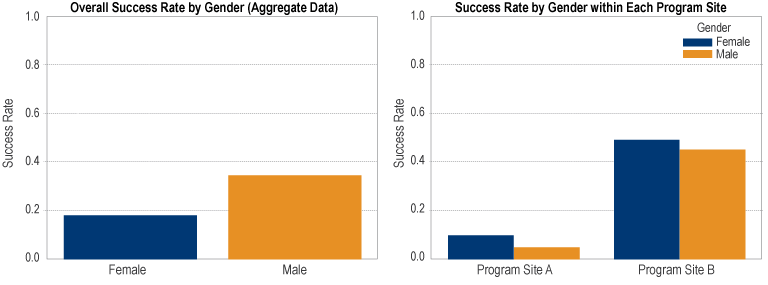
Even when we shouldn’t expect fundamental differences, as in my example, we need explicit causal models of the reasons that apparent differences arise anyway. There is nothing at all controversial about this fact: it arises from the logic of inference about units that have multiple group-level features, that is, multivariate statistics. It is a frequent occurrence in statistical models that disparities emerge only after controlling for relevant characteristics and disparities that appear simply by splitting the data by a single demographic variable disappear or reverse (Simpson’s Paradox, as shown below).
Implicit Standards
Keeping in mind these cautions, what can we do with apparent disparities? I’d like to suggest that noticing a disparity is an excellent way to begin the process of setting a standard. However, the process is far from automatic and we need to keep our wits about us to avoid rushing to “obvious” conclusions. Let’s work through an example. Suppose that an American city notes that the rate of substance use disorder is 6% for women and 12% for men locally – a large disparity. Is this disparity a problem? In many conversations about disparities, the default assumption is that the grand mean (the mean between groups) is an appropriate policy target. This is usually what is meant by “reducing disparities.” If we aim to simply reduce the disparity, then an increase in the SUD rate for women to 10% and a decrease in the SUD rate among men to 11% will count as progress towards this goal, despite the fact that, assuming a roughly equal gender populations in the city, this actually amounts to many more people overall having a substance use disorder. What went wrong here?
It turns out that what we really wanted was for the SUD rate among men to decrease and for the SUD rate among women to either remain steady or decrease as well. These are the only good outcomes for these groups, provided you agree with my valuation of substance use disorders. Direction matters more than the magnitude of the disparity. Arguably, the disparity between women and men alerted us to the fact that a lower SUD rate is theoretically possible for men because women achieve it. This sort of claim is the main utility of analyzing disparities – to show us what may be possible to achieve under the right circumstances.
If you follow my line of reasoning, notice also that the simple disparity between men and women gives us more information about how to set standards for men (i.e., approximately equal to women) than it does for women – is the rate for SUD among women high or low in this city? To learn this information, we can turn to population-level statistics. Suppose that at the population level in the country, the rate of SUD for women is 8% and the rate of SUD for men is 12%. Now we can revisit our original claim that the local disparity between men and women in the local area is a problem. In fact, the city is pretty typical, and women are even beating the average somewhat. From the vantage point of population level information about the groups, the local disparity we originally uncovered turns out to be unsurprising because these differences are expected in the population. If anything, the city should be praised for having a lower average SUD than the country. But, nothing we just learned prevents the city from setting an even lower target for SUD since, as I mentioned in my previous post, setting standards involves multiple kinds of reasoning: descriptive (which we’ve used here), predictive, and normative. The only thing we shouldn’t do is rush to the conclusion that we would be better off if there were no group differences.
Some Questions for Thinking about Disparities in Evaluation
To help evaluators and their stakeholders think more critically about simple observed disparities, I’ll conclude with some questions that I find useful to ask:
- What are the appropriate standards to set for each group in the disparity analysis, regardless of intergroup differences?
- Do I have evidence of the causal process that produced this disparity or am I just telling a familiar story about how things got this way?
- What background variables could I control for to make this apparent disparity diminish? Does the disparity persist after I try this?
- What are the things that we care most about equalizing in the program (the “equalisandum”)? While conducting our analysis of disparities, did we put most of our effort into those indicators?